Calculation algorithm for complex trajectories

Introduction

In modern petroleum engineering, the development of oil and gas reservoirs increasingly relies on wells with complex trajectories, including inclined, horizontal, and S-shaped wellbores. Such wells significantly increase the contact area with the reservoir, improve drainage efficiency, and enhance hydrocarbon recovery from multilayer formations. However, the evaluation of well productivity in these conditions becomes more challenging due to the combined influence of wellbore geometry, inclination angle, permeability anisotropy, partial penetration of formations, skin effects, and frictional pressure losses within the wellbore.

Classical analytical solutions for inflow performance were originally derived for vertical or horizontal wells and often cannot fully represent the behavior of wells with complex trajectories intersecting multiple productive layers. Therefore, an integrated calculation approach that combines different inflow models and accounts for the spatial geometry of the wellbore is required.

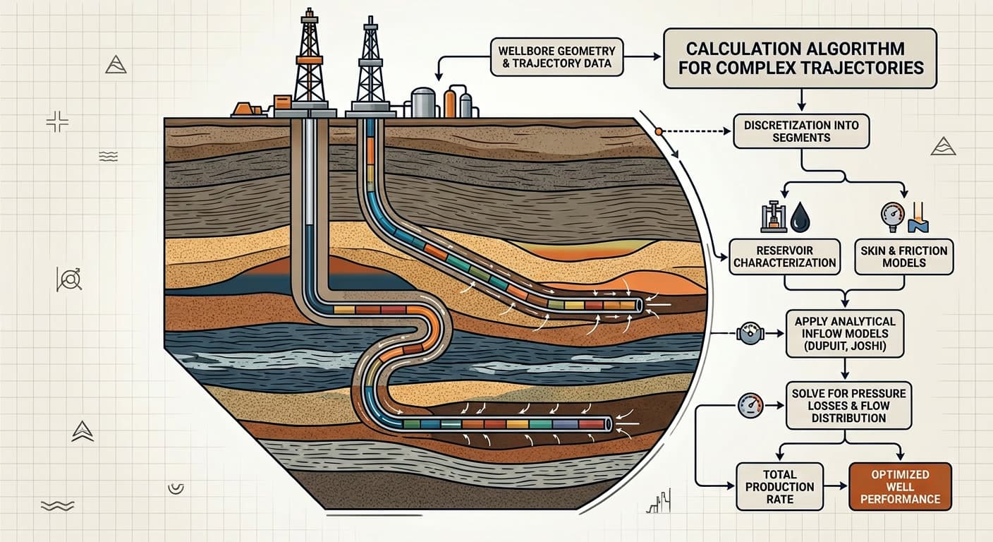
This paper presents a methodology for calculating the productivity of complex-trajectory wells in multilayer reservoirs. The proposed algorithm is based on discretizing the wellbore into segments and applying established analytical models, including the Dupuit solution for radial flow and the Joshi model for horizontal wells, while accounting for skin factors and frictional pressure losses along the wellbore. This approach allows for a more accurate estimation of inflow distribution along the wellbore and the total production rate of the well.

Well Productivity Calculation Method for Complex-Trajectory Wells in Multi-Layer Reservoirs

This methodology describes the algorithm for determining the productivity of wells with complex trajectories (inclined, horizontal, S-shaped) that intersect multiple isolated productive formations, accounting for wellbore inclination angle, anisotropy, skin factors, and frictional pressure losses in the wellbore.

The approach relies on classical solutions for inflow to vertical and horizontal wells (Dupuit, Joshi, Economides) and correlations for skin factors in deviated wells (Cinco-Ley, Besson, and subsequent generalizations).

1. Inflow Calculation for Deviated Wells (Directional Wells)

For wellbore segments where the inclination angle lies outside the horizontal range, the flow pattern approximates radial, and the Dupuit formula for steady-state inflow to a vertical well is applied:

$$q = \frac{2\pi kh\Delta P}{\mu B\left(\ln\left(\frac{R_{e}}{r_{w}}\right) - 0.75 + S_{total}\right)}$$

where:

• k — formation permeability (mD, converted to m² for calculations);
• h — effective formation thickness (m);
• $\Delta P = P_{res} - P_{wf}$ — drawdown (atm or Pa, depending on units);
• $\mu$ — oil viscosity (mPa·s → Pa·s);
• B — oil formation volume factor (dimensionless);
• $R_{e}/r_{w}$ — drainage radius to wellbore radius ratio;
• $S_{total}$ — total skin factor (see Section 3 ).

The classical constant in the denominator corresponds to the pseudoskin factor for radial inflow to a perfectly penetrating vertical well and is documented, e.g., by Economides et al.

2. Inflow Calculation for Horizontal Wells

For segments with inclination angle θ from 80° to 90° (near-horizontal wellbore), the Joshi model for steady-state inflow to a horizontal well in an anisotropic formation is used:

$$q = \frac{kh\Delta P}{\mu B D_{enom}}$$

where the denominator $A\ln\left(\frac{r_{eH}}{r_{w}}\right) + s$ accounts for elliptical drainage geometry and formation anisotropy:

1. Major semi-axis of the ellipse (α):

$$a = \frac{L}{2}\left[0.5 + \sqrt{0.25 + \left(\frac{2r_e}{L}\right)^4}\right]^{0.5}$$

2. Anisotropy coefficient (β) (introduced as $I_{ani}$ or permeability ratio):

$$\beta = \sqrt{\frac{k_h}{k_v}} \text{ or } \beta = \sqrt{I_{ani}}$$

3. Effective thickness (h′):

$$h^{\prime} = h \cdot \beta$$

4. Joshi logarithmic terms (in one common form):

$$\begin{aligned} \ln_1 &= \ln\left(\frac{a}{L/2} + \sqrt{\left(\frac{a}{L/2}\right)^2 - 1}\right) \\ \\ \ln_2 &= \ln\left(\frac{h^{\prime}}{L} \cdot \frac{1 + \beta}{\beta}\right) \\ \\ \ln_3 &= \ln\left(\frac{h^{\prime}}{2r_w} \cdot \sqrt{\frac{h^{\prime}}{L} \cdot \frac{1 + \beta}{\beta}}\right) \end{aligned}$$

Then:

$$\mathit{Denom} = \ln_1 + \ln_2 - \ln_3 + S$$

where s— skin factor (mechanical + other components, see Section 3 ).

The Joshi model is detailed in Horizontal Well Technology and generalized for various drainage geometries in Petroleum Production Systems.

3. Skin Factor Calculations

The total skin factor for each wellbore segment is treated as an additive quantity:

$$S_{total} = S_{mech} + S_{\theta} + S_{p}$$

3.1. Mechanical Skin Factor $S_{mech}$

$S_{mech}$ reflects filtration resistance due to near-wellbore zone contamination by drilling fluid filtrate, perforation damage, uneven penetration, etc. Its value is typically calibrated from well test (WDT/PLT) data or taken from standard correlations (Economides, Babu-Odeh, etc.).

3.2. Inclination Angle Skin Factor

For deviated sections $(0 < θ < 90°)$, the geometric pseudoskin correlation for deviated wells by Cinco-Ley and Besson is used:

$$S_{\theta} = \frac{h}{r_w} \cdot \sqrt{\frac{k_v}{k_h}} \cdot \frac{|\cos \theta|}{41 - 2 \cdot \left(h / R_e\right)}$$

• As $θ → 90°$, $S_{θ}$ transitions to the geometric component of the Joshi model (horizontal well);
• With increasing anisotropy $(k_{v}/k_{h} ≪ 1)$ the inclination effect on $S_{θ}$ grows, confirmed by classical Besson work and modern deviated well correlations.

3.3. Partial Penetration Skin Factor $S_{p}$

The partial penetration skin factor accounts for additional inflow resistance arising when the wellbore intersects only part of the effective formation thickness $h$ and terminates within the formation.

In this case, streamlines converge toward the ends of the open interval, increasing drawdown compared to a fully penetrating well.

To quantify this effect, the widely cited analytical approximation by Papatzacos (1987) is applied, commonly used in inflow analysis and well test interpretation for partially penetrated and perforated intervals.

Calculation Algorithm $S_{p}$:

1. Dimensionless Thickness $h_{D}$

$$h_{D} = \frac{h}{r_w} \cdot \sqrt{\frac{k_h}{k_v}}$$

where $k_h, k_v$ are horizontal and vertical permeabilities, and $r_w$ is the wellbore radius.

2. Geometric Parameter $b$

The parameter $b$ describes the geometry of the partially penetrated interval relative to formation boundaries and accounts for flow asymmetry when the open interval is offset from the formation center:

$$b = \frac{h / h_p}{2 + h / h_p} \cdot \sqrt{\frac{\left(z_w + h_p / 4\right)\left(h - z_w + h_p / 4\right)}{\left(z_w - h_p / 4\right)\left(h - z_w - h_p / 4\right)}}$$

where:

• $h_p$ is the penetrated (perforated) formation thickness;
• $z_w = h - h_p / 2$ is the coordinate of the open interval midpoint relative to the formation top.

3. Final Formula $S_{p}$

$$S_{p} = \left(\frac{h}{h_p} - 1\right) \cdot \ln\left(\frac{\pi \cdot h_D}{2}\right) + \frac{h}{h_p} \cdot \ln(b)$$

The first term reflects the effect of the full-to-penetrated thickness ratio $h / h_p$ and anisotropy via $h_D$, while the second provides a correction for interval position within the formation via $b$. When $h_p \to h$ and the interval is symmetrically centered, $S_p$ is consistent with solutions for fully penetrating wells.

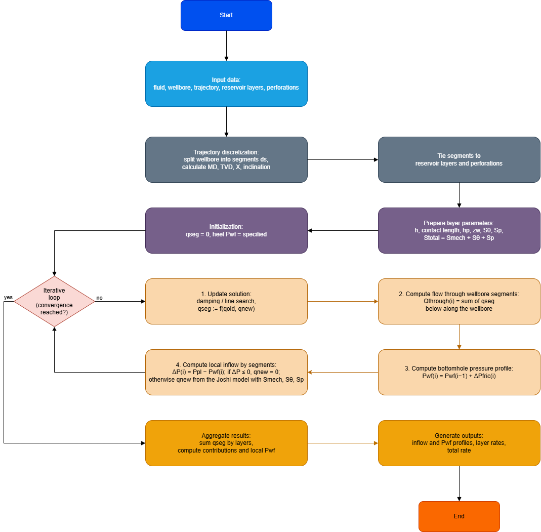
4. Calculation Algorithm for Complex Trajectories (Radial Channel Model)

For wells with curved trajectories crossing multiple layers, a segmented approach (discretized wellbore/segment model) is applied.

Stage 1: Wellbore Discretization

1. Wellbore is divided into segments of length $\Delta L$ (typically 5-10 m; step selected based on trajectory smoothness and logging/inclinometry resolution).
2. For each segment $i$, from inclinometry data:

• average inclination angle $\theta_i$;
• coordinates and affiliation to specific formation $j$;
• local petrophysical parameters $(k_j, h_j, p_{res,j})$.

Stage 2: Calculation Model Selection by Angle

For each segment, the inflow model is selected:

• If $70^\circ \le \theta_i \le 120^\circ$: use Joshi horizontal well model ( Section 2 );
• If $\theta_i < 70^\circ$ or $\theta_i > 120^\circ$: use Dupuit formula ( Section 1 ) with $S_{total}$, including $S_{\theta}$.

For segments partially penetrating the formation, $S_p$ is additionally calculated (see 3.3).

Stage 3: Accounting for Frictional Losses in Wellbore

Drawdown for segment $i$ is determined as:

$$\Delta P_i = P_{res,j} - \left(P_{wf,heel} + \Delta P_{fric,i}\right)$$

where $\Delta P_{fric,i}$ is the frictional pressure loss in the wellbore section from segment $i$ to the heel.

Frictional losses can be estimated using the Darcy-Weisbach equation or standard pipeline correlations (depending on flow regime and phase composition), using current total flow rate in that wellbore section.

The general solution is iterative:

1. Assign initial flow rate distribution across segments, for example proportional to $k \cdot h$.
2. Calculate $\Delta P_{fric,i}$ along the wellbore.
3. Recalculate $\Delta P_i$ and inflow $q_{i,j}$ using Dupuit/Joshi models.
4. Repeat until convergence on total flow rate and bottomhole pressure $P_{wf}$.

This approach is described in IPR studies for horizontal/deviated wells, where neglecting friction leads to overestimation of productivity and errors in water/gas breakthrough timing.

Stage 4: Summing Flow Rates

Total well flow rate:

$$Q_{total} = \sum_{j=1}^{n} \sum_{i=1}^{m_j} q_{i,j}$$

where:

• $j$ is the formation (layer) index;
• $i$ is the segment index belonging to layer $j$;
• $q_{i,j}$ is the inflow from segment $i$ of layer $j$, calculated by the selected model.

Additionally, an inflow profile along the wellbore and by layers can be generated to assess penetration efficiency and identify zones with excessive resistance (high $S_{total}$).

References

1. Joshi S. D. Horizontal Well Technology. PennWell Publishing Company, 1991.
2. Economides M. J., et al. Petroleum Production Systems. Prentice Hall, 1994.
3. Cinco-Ley H., Samaniego F. “Transient Pressure Analysis for Fractured Wells.” JPT, 1981.
4. Besson J. “Performance of Slanted and Horizontal Wells.” SPE 20965, SPERE, 1990.
5. Modern reviews on IPR for horizontal wells and wellbore friction effects.

Case Study: Application of a Segmented Well Modeling Approach for Productivity Evaluation of an S-Shaped Well

As a representative example, a scenario is considered to demonstrate the impact of well trajectory on the inflow profile. Three hydraulically isolated reservoir layers exhibit identical petrophysical and flow properties; however, they intersect the wellbore with different geometrical configurations. A comparison between the segmented well modeling approach and a simplified layer-based analytical model reveals not only significant quantitative discrepancies but also a qualitative distortion of the physical representation of the inflow distribution.

Problem Definition and Input Data

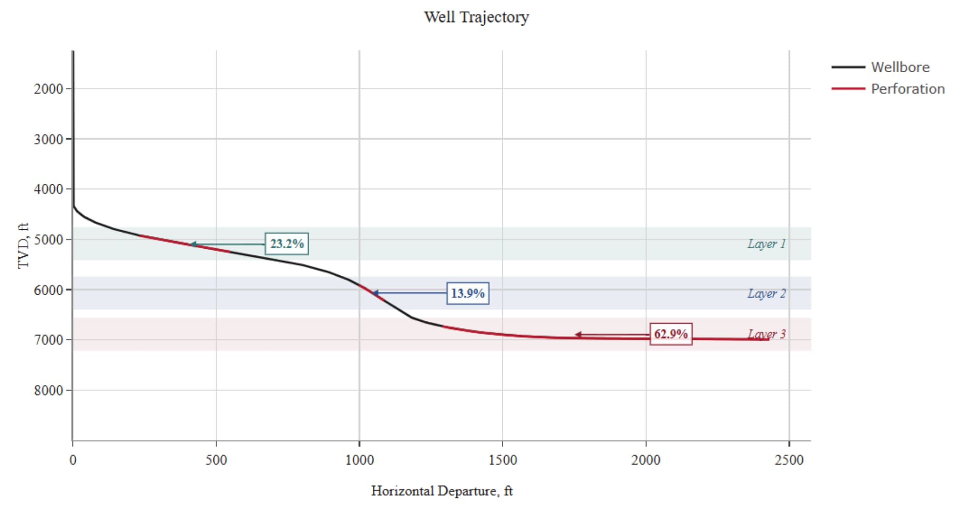
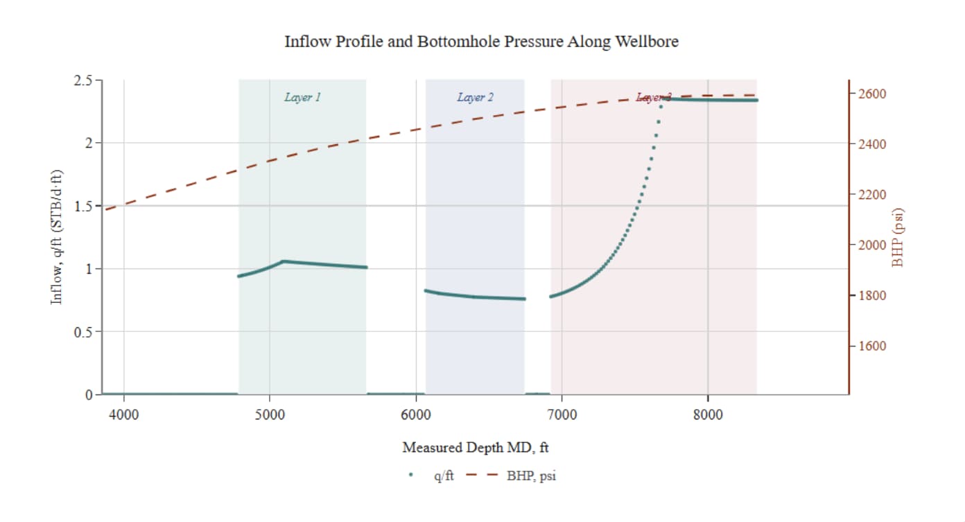
An S-shaped well intersecting three productive reservoir layers is considered. The layers have identical properties: permeability of 100 mD, permeability anisotropy defined by the ratio $k_{v} / k_{h} = 0.30$, reservoir pressure of 270 atm, and mechanical skin factor $S_{mech}$. The wellbore diameter is 0.05 m, and the bottomhole pressure at the heel is 100 atm. Each layer has a thickness of 200 m, with the perforated interval located at the center and equal to 100 m (50% reservoir penetration, Figure 1).

The segmented approach represents the wellbore as a discrete set of segments. For each segment, the inclination angle, reservoir layer assignment, and local properties are determined from trajectory (inclination survey) data. An appropriate inflow model (radial or quasi-horizontal) is then selected, and skin components are incorporated, including mechanical skin, angular pseudoskin, and partial penetration skin. The local pressure drawdown is subsequently updated iteratively, accounting for cumulative pressure losses along the wellbore. 1, 2

Simulation Results and Inflow Redistribution Analysis

According to the segmented well model, the production rates from the reservoir layers are 143.7, 86.0, and 389.7 m³/day, respectively, resulting in a total well production rate of 619.5 m³/day. The fractional contribution of each layer to the total inflow is 23.2%, 13.9%, and 62.9%, respectively (Figure 2).

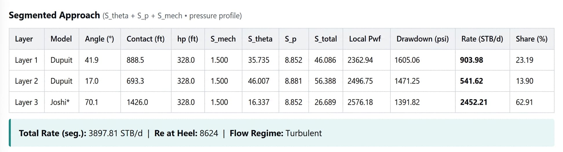
Since the petrophysical properties of the reservoir layers are identical, the non-uniform inflow profile is solely governed by the wellbore spatial configuration and wellbore hydraulic losses. The intersection geometry is characterized by average inclination angles of 41.9°, 17.0°, and 70.1° for the respective layers. This spatial orientation results in angular pseudoskin values $S_{θ}$ of 35.75, 45.95, and 16.35, respectively. The partial penetration skin factor $S_{p}$ is identical for all layers (8.85), reflecting the same relative geometry of the perforated intervals [5].

The physical mechanism underlying this phenomenon follows a clear cause-and-effect relationship: wellbore geometry determines the local pseudoskin, which directly controls the near-wellbore flow resistance and, consequently, leads to a nonlinear redistribution of formation inflow. In steady-state flow equations, the flow resistance appears in the denominator of a logarithmic function involving flow geometry parameters and the skin factor. An increase in the total skin (S) results in a proportional reduction of the productivity index (PI) [3]. For inclined and horizontal completions, geometric effects become dominant: the effective flow resistance critically depends on the inclination angle and permeability anisotropy [4].

Superposition of all skin components (mechanical, angular, and partial penetration) for the considered layers yields total skin values of 46.1, 56.3, and 26.7. Thus, the overall flow resistance of the second layer exceeds that of the third layer by more than a factor of two, despite the mechanical formation damage being only 1.5. Therefore, well trajectory effects dominate over classical near-wellbore formation damage (formation impairment) effects.

Impact of Wellbore Hydraulic Losses on Local Pressure Drawdown

A critically important physical mechanism captured by the segmented well model is the degradation of local pressure drawdown due to frictional pressure losses along the wellbore. In the considered case, the local flowing bottomhole pressure $P_{wf}$ increases from 160.85 atm in the upper (first) layer to 175.37 atm in the lower (third) layer. The resulting longitudinal pressure gradient of approximately 14.5 atm leads to a proportional reduction in local pressure drawdown from 109.15 to 94.63 atm (Figure 3).

In engineering literature, this phenomenon is classified as a macroscopic manifestation of the heel-toe effect: frictional pressure losses along an extended wellbore section create a pressure differential between the heel and the toe, resulting in an asymmetric inflow profile even in a homogeneous reservoir [6, 7]. From a pipeline hydraulics perspective, distributed friction losses are described by the Darcy–Weisbach equation [8]. In this context, a horizontal well can be treated as a system with distributed inflow (“pipe manifold with T-junctions”), where continuous fluid influx from the reservoir dynamically alters the velocity profile along the wellbore, requiring a coupled solution of wellbore flow equations and reservoir flow (filtration) equations [9, 10].

Comparison with a Layer-Based Analytical Model (Simplified Approach)

The conventional layer-based analytical approach assumes averaged reservoir properties and neglects pressure gradients within the wellbore. Under identical values of $k$, $h$, and ${\Delta P}$, and considering only the mechanical skin $S_{mech}$, the first and second layers produce identical inflow. Within this framework, the predicted production rates are 928.2, 928.2, and 518.2 m³/day, respectively, resulting in a total well production rate of 2374.6 m³/day (Figure 4).

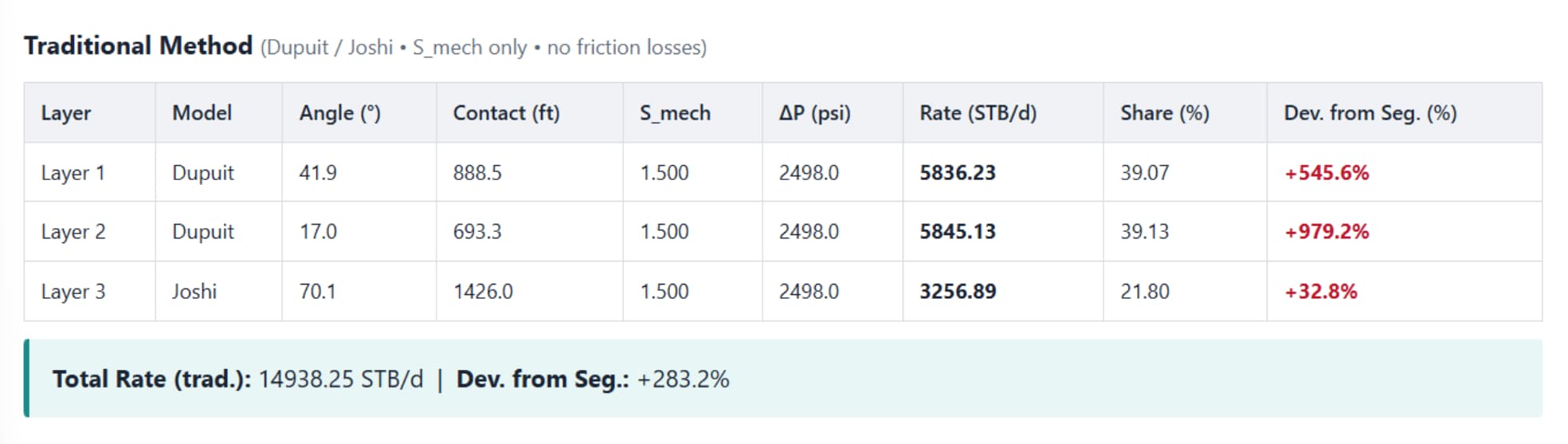
Comparison with the segmented well model results (619.5 m³/day) shows that the simplified analytical model overestimates well productivity by a factor of 3.83 (error of +283%). This significant discrepancy is explained by the underlying assumptions of the layer-based model: neglect of angular pseudoskin, omission of additional flow resistance due to partial penetration, and the assumption of uniform (isobaric) pressure along the wellbore.

In classical IPR models for horizontal wells, the inability to properly account for frictional pressure losses is a well-known limitation [11]. The use of the Joshi formulation in its basic form assumes an equipotential wellbore wall, which is not valid in the presence of a significant pressure gradient along the wellbore length [12].

Discussion

The obtained results clearly demonstrate the fundamental limitations of conventional analytical approaches that rely on an average inclination angle and an equivalent drainage radius when applied to multilayer wells with complex trajectories. The segmented analysis shows that under anisotropic reservoir conditions $k_{v} / k_{h} < 1$, the local wellbore orientation (inclination angle) exerts a disproportionately strong influence on flow resistance. In particular, the angular pseudoskin in inclined intervals may exceed the mechanical skin $S_{mech}$ by an order of magnitude, becoming the primary limiting factor for well productivity.

Furthermore, the study confirms that neglecting wellbore hydrodynamics (frictional effects) inevitably leads to overestimation of the effective pressure drawdown in distal (toe) sections. This not only distorts the predicted total production rate but also results in an incorrect representation of the inflow profile along the wellbore. The practical implications are particularly significant for well completion design: accurate prediction of the heel-toe effect is essential for proper design of inflow control devices (ICD/AICD), optimization of liner diameters, and mitigation of premature water or gas coning in zones of excessive drawdown near the heel.

Conclusions and Practical Recommendations

1. Non-uniform inflow profile. In wells with complex architectures draining multilayer reservoirs, the inflow profile is governed not only by reservoir transmissibility $kh$ but also, to a significant extent, by completion geometry (local inclination angle and penetration ratio). Reservoir layers with identical properties may exhibit substantially different contributions to total production.
2. Dominance of geometric pseudoskin. The angular skin factor $S_{θ}$ and the additional flow resistance associated with partial penetration $S_{p}$ may exceed conventional mechanical skin $S_{mech}$ by several times. Well trajectory geometry thus becomes the primary factor controlling near-wellbore flow resistance.
3. Importance of wellbore hydraulic losses (heel-toe effect). Frictional forces in deviated and horizontal sections may cause a significant increase in bottomhole pressure from heel to toe in long, high-productivity wells, leading to a reduction of effective pressure drawdown in distal intervals. Iterative coupling of wellbore hydraulics is therefore essential to ensure the physical consistency of the model.
4. Limitations of layer-based analytical models. The use of classical simplified approaches that do not account for discrete inflow distribution and wellbore pressure losses leads to a significant overestimation of predicted well productivity (up to 280%) and distortion of the inflow profile. For the design of S-shaped and horizontal wells, as well as wells with radial laterals of varying lengths, the segmented well modeling approach should be considered a standard engineering practice.

References

• [1] [2] [10] [16] - Optimization of Horizontal Well Completion
• [3] [14] - PETROLEUM PRODUCTION SYSTEMS
• [4] - Performance of Slanted and Horizontal Wells on an Anisotropic Medium
• [5] - Approximate partial-penetration pseudoskin for infinite-conductivity wells
• [6] [9] [13] [15] [17] - A novel analytical approach to design horizontal well completion using ICDs to eliminate heel-toe effect
• [7] [11] - Effects of Pressure Drop in Horizontal Wells and Optimum Well Length
• [8] - State-of-the-art Review on Measurement of Pressure Losses of Fluid Flow through Pipe Fittings
• [12] - Inflow Performance of a Cyclic-Steam-Stimulated Horizontal Well Under the Influence of Gravity Drainage